4. Some other common univariate distributions

1. Student \( t \) distribution

Gaussian은 tail에 mass가 많지 않아서 outlier에 민감한 편이다.
Gaussian과 비슷하지만 outlier에 덜 민감한 distribution으로 student \( t \) distribution을 들 수 있다.

\[\mathcal{T}(y|\mu, \sigma^2, \nu) \propto [1 + \frac{1}{\nu}(\frac{y - \mu}{\sigma})^2]^{(\frac{\nu + 1}{2})} \qquad{(3.60)}\]

위 distribution의 파라미터들을 살펴보자
1. \( \mu \): mean 값
2. \( \sigma > 0 \): scale parameter
3. \( \nu > 0 \): degree of freedom 또는 degree of normality. 후자의 명칭은 값이 클수록 normal distribution에 가까워지기 때문이다.
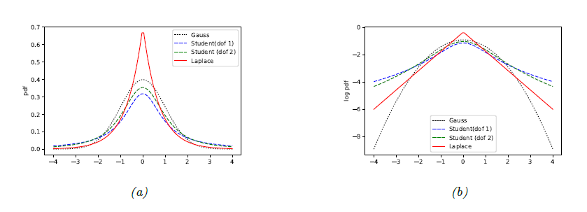
gaussian이 mean값에서 멀어지면서 exponentially decay하는데에 비해, 식에서 알 수 있듯이 이 distribution은 polynomial function으로 decay한다.
따라서 gaussian보다 heavy tail을 갖는다고 표현한다.

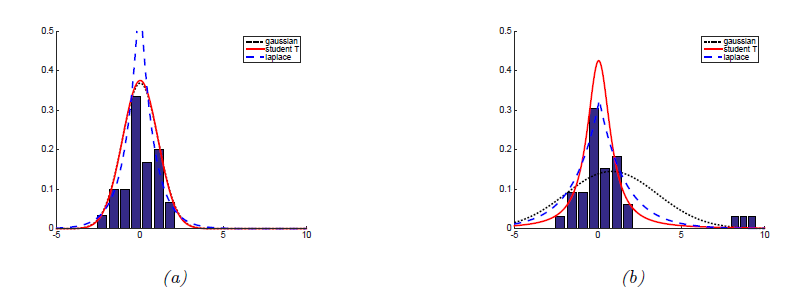
마찬가지로, 위 그림에서는 outlier가 없을때와 있을 때 얼마나 distribution이 sensitive하게 변하는지를 볼 수 있다. Gaussian은 민감하게 변하는데에 비해 student-t는 그렇지 않음을 알 수 있다.
아래와 같은 특징이 있다.

\[\mathrm{mean} = \mu, \, \mathrm{mode} = \mu, \, \mathrm{var} = \frac{\nu\sigma^2}{(\nu - 2)} \qquad{(3.61)}\]

\( \nu > 1 \) 일때만 mean 값이 정의되고, variance는 \( \nu > 2 \) 일 때만 정의된다.
\( \nu \) 의 값이 커질수록 gaussian에 가까워 지기때문에 outlier에 대한 robustness가 점점 감소하게 되며, \( \nu = 4 \)의 값을 모델링에 많이 이용한다.

student distribution의 \( \nu \)값이 1일 경우에는 어떤 distribution일까? 이를 Cauchy distribution 혹은 Lorentz distribution이라고 한다.

\[\mathcal{C}(x|\mu, \gamma) = \frac{1}{\gamma\pi} \Big[ 1 + \Big(\frac{x - \mu}{\gamma}\Big)^2 \Big]^{-1} \qquad{(3.62)}\]

student t 중 가장 normality가 낮다
- 결국 tail에 가장 많은 weight이 실려있고, 따라서 mass가 많이 퍼져있다는 것을 알 수 있다.
- 직관적인 예로, gaussian에서의 \( z = (-1.96, 1.96)) \) 인터벌이 Cauchy에서는 \( z = (-12.7, 12.7)) \)에 해당한다.
Half-normal처럼 Half-Cauchy도 존재한다.
- 나중에 Bayesian modeling에 쓰인다.

Laplace distribution은 figure 3.8에서 볼 수 있는것처럼 가운데에 피크가 높게 뜨고, 대신에 tail에 있는 mass도 gaussian보다 높다. 단지 mode에서 가까운 값에서 더 가파르게 떨어진다.
- 이렇게 exponentially 감소하는 property 때문에 double-sided exponential distribution이라고 불리기도 한다.

\[\mathrm{Lap}(y|\mu, b) := \frac{1}{2b} \exp \Big(-\frac{|y - \mu|}{b})\Big) \qquad{(3.64)}\]

위와 같은 식을 가지며, 여기서 \( \mu \)는 mode를 좌우하고 \( b \)는 scale parameter로 variance를 좌우한다.
아래와 같은 특징을 갖는다.

\[\mathrm{mean} = \mu, \, \mathrm{mode} = \mu, \, \mathrm{var} = 2b^2 \qquad{(3.65)}\]

\[\mathrm{Beta}(x|a,b) = \frac{1}{B(a,b)}x^{a-1}(1-x)^{b-1} \qquad{(3.66)}\]

\[B(a,b) := \frac{\Gamma(a)\Gamma(b)}{\Gamma(a+b)} \qquad{(3.67)}\]

\[\Gamma(a) := \int_0^\infty x^{a-1}e^{-x}dx \qquad{(3.68)}\]

위 그림의 (a)는 beta distribution을 나타내는데, 보이다시피 \( a = 1, b = 1 \)일 때는 uniform distribution과 equivalent하다.
- 좀 당황스럽긴 하지만, 많은 딥러닝 논문에서 Beta distribution에서 특정 파라미터 값을 샘플링 해놨다고 해놓고 \( a = b = 1 \)인 beta distribution에서 샘플링했다고 하는 경우가 있는데, 속지 말자
\( a,b > 0 \) 이라는 조건을 만족해야 integrable하다.
\( a,b < 1 \) 인 경우 0과 1에서 peak를 갖는 bimodal distribution이 형성된다.
\( a,b > 1 \) 인 경우 가운데가 볼록한 unimodal distribution이 만들어진다.
아래와 같은 property를 갖는다.

\[\mathrm{mean} = \frac{a}{a+b}, \, \mathrm{mode} = \frac{a-1}{a+b-2}, \, \mathrm{var} = \frac{ab}{(a+b)^2(a+b+1)} \qquad{(3.69)}\]

postive, real valued random variable을 위한 pdf이다.
두 가지 다른 paramter가 있다.
- \( a > 0 \): shape parameter
- \( b > 0 \): rate parameter

\[\mathrm{Ga}(x|a,b) := \frac{b^a}{\Gamma(a)}x^{a-1}e^{-xb} \qquad{(3.70)}\]

\[\mathrm{mean} = \frac{a}{b}, \, \mathrm{mode} = \frac{a-1}{b}, \, \mathrm{var} = \frac{a}{b^2} \qquad{(3.72)}\]

\[\mathrm{Expon(x|\gamma)} := \mathrm{Ga}(x|a = 1, b =\gamma) \qquad{(3.73)}\]

shape parameter = 1인 경우로, Poisson process에서 event 사이의 time을 나타내는 것으로 알려져있다.
memory-less property또한 중요한데, 어느 지점에서 distribution을 시작해도 항상 동일한 distribution으로 볼 수 있다는 뜻이다. exponential function인 것을 고려하면 trivial하다.

\[\chi^2_\nu(x) := \mathrm{Ga}(x|a = \frac{\nu}{2},b= \frac{1}{2}) \qquad{(3.74)}\]